Learning, under
the microscope.
A field guide to the experiment you can change.
Every image below comes from the bundled, reproducible model.
Give a line
somewhere to bend.
In XOR, opposite corners share a class. A classifier whose score is a linear combination of x₁ and x₂ cannot draw the boundary this pattern needs. Adding hidden units with nonlinear activations changes the functions the network can represent. Merely stacking linear layers would still leave a linear function. Google’s neural-network lesson ↗
Try it: open the guided tour. The lab brings the plot and live readouts together in focus view. Fit the linear model, then add the 6 → 4 hidden layers. Compare their boundaries at the same epoch.
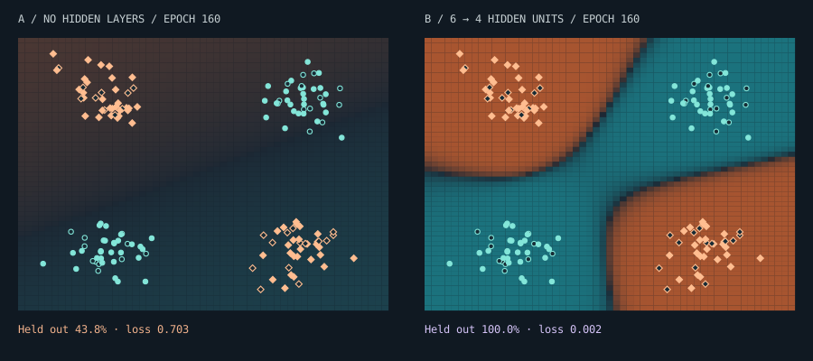
Many simple fields.
One learned decision.
Click a neuron thumbnail, then Neuron lens. The landscape now shows that neuron’s activation, rather than the final probability. First-layer units respond to weighted sums of x₁ and x₂; later units combine earlier responses. An activation field describes a numerical response, not a human concept.
Follow a point using the landscape or the point selector. Expand All layer values & gradients to see each preactivation z, activation a, and derivative δ = ∂loss/∂z. Input rows show ∂loss/∂x. These derivatives describe one point, without jitter or L2; a held-out point’s derivatives are diagnostic only.
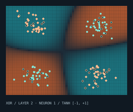
Perfect on the past.
Less certain elsewhere.
A falling training loss can coexist with a rising validation loss. That divergence can indicate overfitting: the model fits the observations it learned from at the expense of unseen observations. Google’s overfitting lesson ↗
Try it: choose Compare experiments → Try the overfitting experiment. Both 16 → 16 models train on the same noisy clusters. B penalizes large weights with L2. That can limit complexity; its strength still needs to be chosen for the problem. L2 regularization ↗
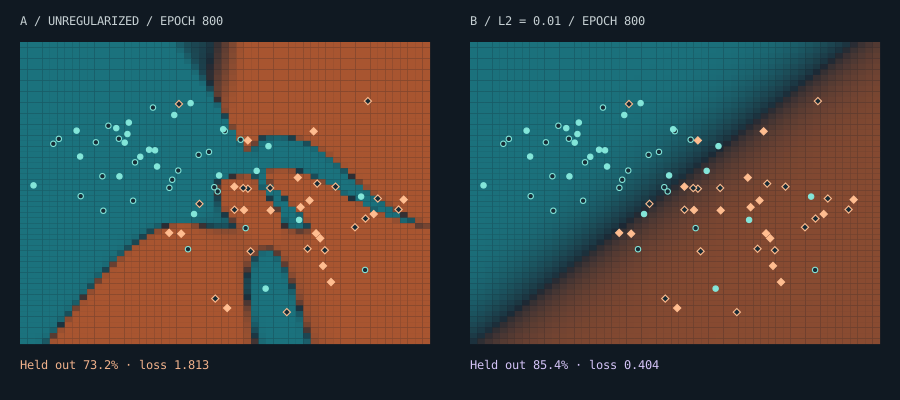
“Held out” here means a validation set. Repeatedly using it to choose settings influences model selection. This lab has no independent final test set, and confidence between points is not a guarantee of correctness.
The arithmetic
behind the image.
The model takes two coordinates and predicts the probability of class B. The output uses a sigmoid. The plotted loss is mean binary cross-entropy, evaluated on the original, unperturbed points. It excludes the regularization penalty so A and B are comparable.
Biases are not penalized. Accuracy uses P(B) ≥ 0.5.
One epoch is one full-batch update. The optimizer is Adam, with β₁ = 0.9, β₂ = 0.999, ε = 10⁻⁸ and bias correction. The global gradient norm is clipped to 5 before an update. Kingma & Ba, Adam (2015) ↗
Input jitter adds independent Gaussian noise with standard deviation 0.06 to training coordinates only. “Noisy clusters” separately includes a 10% probability of a label flip. Splits are seeded and stratified; rounding can make a 50% split differ by one point per class.
A result you
can pick up again.
Export weights + data, then Download session. The JSON contains points, split assignments, weights, Adam moments, epoch, and random state. Import restores predictions and continuation. Historical curves restart at the imported checkpoint: old curve claims are not trusted as measured evidence.
Reset returns to the same seed and dataset. Drawing pauses training and resets weights after the stroke; it preserves existing split assignments. Choose the held-out set before drawing observations that should never train the model.
Try these measured checkpoints with Import session:
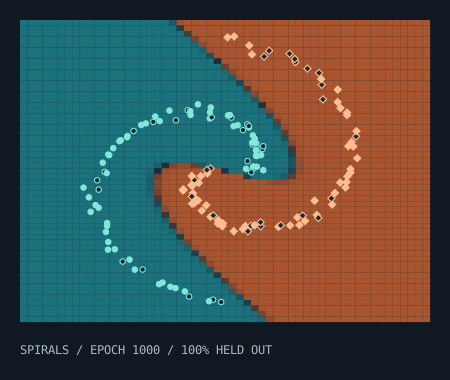
- 00–10sOpen the guided tour. Point out the alternating XOR corners.
- 10–20sTrain the straight line. Its geometry cannot separate XOR.
- 20–35sAdd hidden layers. Watch B’s curved decision boundary emerge beside A.
- 35–45sLook through a neuron, then follow a point and expand its gradients.
- 45–60sReturn to the landscape. Export the exact experiment as JSON.
Small by design
At most 320 observations, three hidden layers of 16 units, two experiments, and 3,000 epochs. One worker, no remote inference. Training pauses when hidden and requires an explicit resume. Fields sample a 73 × 73 lattice and interpolate spatially; values update about six times per second. Curves sample every eight updates, plus the current endpoint.
These are synthetic two-dimensional classification experiments. They explain useful mechanisms without reproducing frontier-model training or establishing performance on real-world data.
Start an experiment →